Building the Canonical sample

According to the nomenclature used in Ishida et al., 2019, the Canonical sample is a subset of the test sample chosen to hold the same characteristics of the training sample. It was used to mimic the effect of continuously adding elements to the training sample under the traditional strategy.

It was constructed using the following steps:

1. From the raw light curve files, build a metadata matrix containing: [snid, sample, sntype, z, g_pkmag, r_pkmag, i_pkmag, z_pkmag, g_SNR, r_SNR, i_SNR, z_SNR] where z corresponds to redshift, x_pkmag is the simulated peak magnitude and x_SNR denotes the mean SNR, both in filter x;
2. Separate original training and test set in 3 subsets according to SN type: [Ia, Ibc, II];
3. For each object in the training sample, find its nearest neighbor within objects of the test sample of the same SN type and considering the photometric parameter space built in step 1.

This will allow you to construct a Canonical sample holding the same characteristics and size of the original training sample but composed of different objects.

actsnclass allows you to perform this task using the py:mod:actsnclass.build_snpcc_canonical module:

>>> from snactclass import build_snpcc_canonical

>>> # define variables
>>> data_dir = 'data/SIMGEN_PUBLIC_DES/'
>>> output_sample_file = 'results/Bazin_SNPCC_canonical.dat'
>>> output_metadata_file = 'results/Bazin_metadata.dat'
>>> features_file = 'results/Bazin.dat'

>>> sample = build_snpcc_canonical(path_to_raw_data: data_dir, path_to_features=features_file,
>>>                               output_canonical_file=output_sample_file,
>>>                               output_info_file=output_metadata_file,
>>>                               compute=True, save=True)

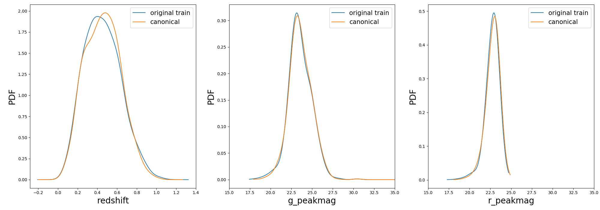
Once the samples is constructed you can compare the distribution in [z, g_pkmag, r_pkmag] with a plot:

>>> from actsnclass import plot_snpcc_train_canonical

>>> plot_snpcc_train_canonical(sample, output_plot_file='plots/compare_canonical_train.png')

In the command line, using the same parameters as in the code above, you can do all at once:

>>> build_canonical.py -c <if True compute metadata>
>>>       -d <path to raw data dir>
>>>       -f <input features file> -m <output file for metadata>
>>>       -o <output file for canonical sample> -p <comparison plot file>
>>>       -s <if True save metadata to file>

You can check that the file results/Bazin_SNPCC_canonical.dat is very similar to the original features file. The only difference is that now a few of the sample variables are set to queryable:

id redshift type code sample gA gB gt0 gtfall gtrise rA rB rt0 rtfall rtrise iA iB it0 itfall itrise zA zB zt0 ztfall ztrise
116537 0.5547 II 36 test 10.969309008063526 -2.505571025776927 33.36879338510094 89.92091344407919 -1.4070121479476083 35.57261257957346 -0.97172916012906 47.691951316763436 37.48483229249487 -7.146619117223875 41.16723042762342 0.14005823764049471 47.983238664813264 39.02626334489017 -6.096248676680143 36.82968789062783 -0.373638211418927 48.438610651533445 41.8848763303308 -7.169183522127793
855370 0.5421 Ibc 23 test -5.514648646328689 3.370545820694393 6.890703579070343 127.00223553079377 -0.04721760599586505 27.987087830949765 -0.4446376337515848 51.06299616763716 13.46475077451422 -0.7802021055103384 42.50390337399486 1.217778587283846 63.88727539461748 4.425762504064253 -2.826164280709543 57.08358377564619 -0.9866672975549484 65.3976378960504 2.88096954432307 -2.211749860376304
328118 0.3131 II 37 test 28.134338786167365 0.7147372066065217 45.830405214215425 15.850284787778433 -0.0005766632993162762 29.225476277548275 -1.9734118280637896 45.83230493446332 87.25700882127312 -0.00025821702716214264 24.95217257542528 -0.3731568724509137 40.527255841246365 311.42509172517947 -3.099534332677601 46.782672798921226 -0.05678675661798624 53.51739930097104 50.76716462668245 -4.572685479766832
704481 0.4665 Ia 0 queryable -50.86850174812521 2.4148469184147547 16.05240678384717 3.5459318666713298 -0.4734666030325012 74.65602268994473 -3.763616485144308 48.208444944828855 24.3318092539982 -4.452287612782472 83.29745588526693 -7.371877954771961 50.92270461365078 38.76468635410394 -10.931632426569717 73.35112115534632 -1.2509966370291774 40.053959252846106 44.453394158157614 -0.18674652754319326
43679 0.5756 II 33 test 28.24271470397688 -3.438072722932048 23.521675700587007 32.4401288159836 -0.2295765027048151 -37.86668398190429 6.8580060036559365 22.252525376185087 2.3940753934318044 -1.611409074593934 -20.420915833911547 9.2659565057976 7.0218302478113035 23.713442135755557 -0.027609543521757457 14.76124690750807 -5.175821286895905 32.58560788340983 115.86494837233313 -0.2587648450330448
172648 0.7592 II 31 test -5.942021205498 2.5808480681448858 72.24216865162195 83.43696533883242 -0.04052830859563986 17.05919635984848 1.005755998955811 18.148318002391164 33.16119808959254 -0.12803412647871454 12.153694246253906 -1.2962293252577974 17.493068792921502 89.98548146319197 -0.14950758787782462 13.355316206445695 -2.4143982246591293 23.84002028961246 118.87985827861259 -1.4858837093947788
762146 0.7245 Ibc 22 test 10.734014319410377 -0.696725251384634 92.36623187978644 0.5112285753252996 -0.4900012400030447 12.968161724599275 -0.94670057528261 55.7516252880299 25.59410571631452 -1.971658945324412 19.03779421586546 -2.228264147418322 57.66412361316971 35.09222360219662 -3.325944814741228 22.877393161444374 0.3070939958786501 57.9675613727551 49.63155574417528 -1.8832424871891025

This means that you can use the actsnclass.learn_loop module in combination with a RandomSampling strategy but reading data from the canonical sample. In this way, at each iteration the code will select a random object from the test sample but a query will only be made is the selected object belongs to the canonical sample.

In the command line, this looks like:

>>> run_loop.py -i results/Bazin_SNPCC_canonical.dat -b <batch size> -n <number of loops>
>>>             -d <output metrics file> -q <output queried sample file>
>>>             -s RandomSampling -t <choice of initial training>