Active Learning loop

Details on running 1 loop

Once the data has been pre-processed, analysis steps 2-4 can be performed directly using the DataBase object.

For start, we can load the feature information:

>>> from actsnclass import DataBase

>>> path_to_features_file = 'results/Bazin.dat'

>>> data = DataBase()
>>> data.load_features(path_to_features_file, method='Bazin')
Loaded  21284  samples!

Notice that this data has some pre-determine separation between training and test sample:

>>> data.metadata['sample'].unique()
array(['test', 'train'], dtype=object)

You can choose to start your first iteration of the active learning loop from the original training sample flagged int he file OR from scratch. As this is our first example, let’s do the simple thing and start from the original training sample. The code below build the respective samples and performs the classification:

>>> data.build_samples(initial_training='original', nclass=2)
Training set size:  1093
Test set size:  20191

>>> data.classify(method='RandomForest')
>>> data.classprob                        # check classification probabilities
array([[0.461, 0.539],
       [0.346, 0.654],
       ...,
       [0.398, 0.602],
       [0.396, 0.604]])

Hint

If you wish to start from scratch, just set the initial_training=N where N is the number of objects in you want in the initial training. The code will then randomly select N objects from the entire sample as the initial training sample. It will also impose that at least half of them are SNe Ias.

For a binary classification, the output from the classifier for each object (line) is presented as a pair of floats, the first column corresponding to the probability of the given object being a Ia and the second column its complement.

Given the output from the classifier we can calculate the metric(s) of choice:

>>> data.evaluate_classification(metric_label='snpcc')
>>> print(data.metrics_list_names)           # check metric header
['acc', 'eff', 'pur', 'fom']

>>> print(data.metrics_list_values)          # check metric values
[0.5975434599574068, 0.9024767801857585,
0.34684684684684686, 0.13572404702012383]

and save results for this one loop to file:

 >>> path_to_features_file = 'results/Bazin.dat'
 >>> metrics_file = 'results/metrics.dat'
 >>> queried_sample_file = 'results/queried_sample.dat'

>>> data.save_metrics(loop=0, output_metrics_file=metrics_file)
>>> data.save_queried_sample(loop=0, queried_sample_file=query_file,
>>>                          full_sample=False)

You should now have in your results directory a metrics.dat file which looks like this:

day accuracy efficiency purity fom query_id
0 0.4560942994403447 0.5545490350531705 0.23933367329593744 0.05263972502898026 81661

Running a number of iterations in sequence

We provide a function where all the above steps can be done in sequence for a number of iterations. In interactive mode, you must define the required variables and use the actsnclass.learn_loop function:

>>> from actsnclass.learn_loop import  learn_loop

>>> nloops = 1000                                  # number of iterations
>>> method = 'Bazin'                               # only option in v1.0
>>> ml = 'RandomForest'                            # only option in v1.0
>>> strategy = 'RandomSampling'                    # learning strategy
>>> input_file = 'results/Bazin.dat'               # input features file
>>> metric = 'results/metrics.dat'                 # output metrics file
>>> queried = 'results/queried.dat'                # output query file
>>> train = 'original'                             # initial training
>>> batch = 1                                      # size of batch

>>> learn_loop(nloops=nloops, features_method=method, classifier=ml,
>>>            strategy=strategy, path_to_features=input_file, output_metrics_file=metrics,
>>>            output_queried_file=queried, training=train, batch=batch)

Alternatively you can also run everything from the command line:

>>> run_loop.py -i <input features file> -b <batch size> -n <number of loops>
>>>             -d <output metrics file> -q <output queried sample file>
>>>             -s <learning strategy> -t <choice of initial training>

The queryable sample

In the example shown above, when reading the data from the features file there was only 2 possibilities for the sample variable:

>>> data.metadata['sample'].unique()
array(['test', 'train'], dtype=object)

This corresponds to an unrealistic scenario where we are able to obtain spectra for any object at any time.

Hint

If you wish to restrict the sample available for querying, just change the sample variable to queryable for the objects available for querying. Whenever this keywork is encountered in a file of extracted features, the code automatically restricts the query selection to the objects flagged as queryable.

Active Learning loop in time domain

Considering that you have previously prepared the time domain data, you can run the active learning loop in its current form either by using the actsnclass.time_domain_loop or by using the command line interface:

>>> run_time_domain.py -d <first day of survey> <last day of survey>
>>>        -m <output metrics file> -q <output queried file> -f <features directory>
>>>        -s <learning strategy> -t <choice of initial training>

Make sure you check the full documentation of the module to understand which variables are required depending on the case you wish to run.

For example, to run with SNPCC data, the larges survey interval you can run is between 20 and 182 days, the corresponding option will be -d 20 182.

In the example above, if you choose to start from the original training sample, -t original you must also input the path to the file containing the full light curve analysis - so the full initial training can be read. This option corresponds to -t original -fl <path to full lc features>.

More details can be found in the corresponding docstring.

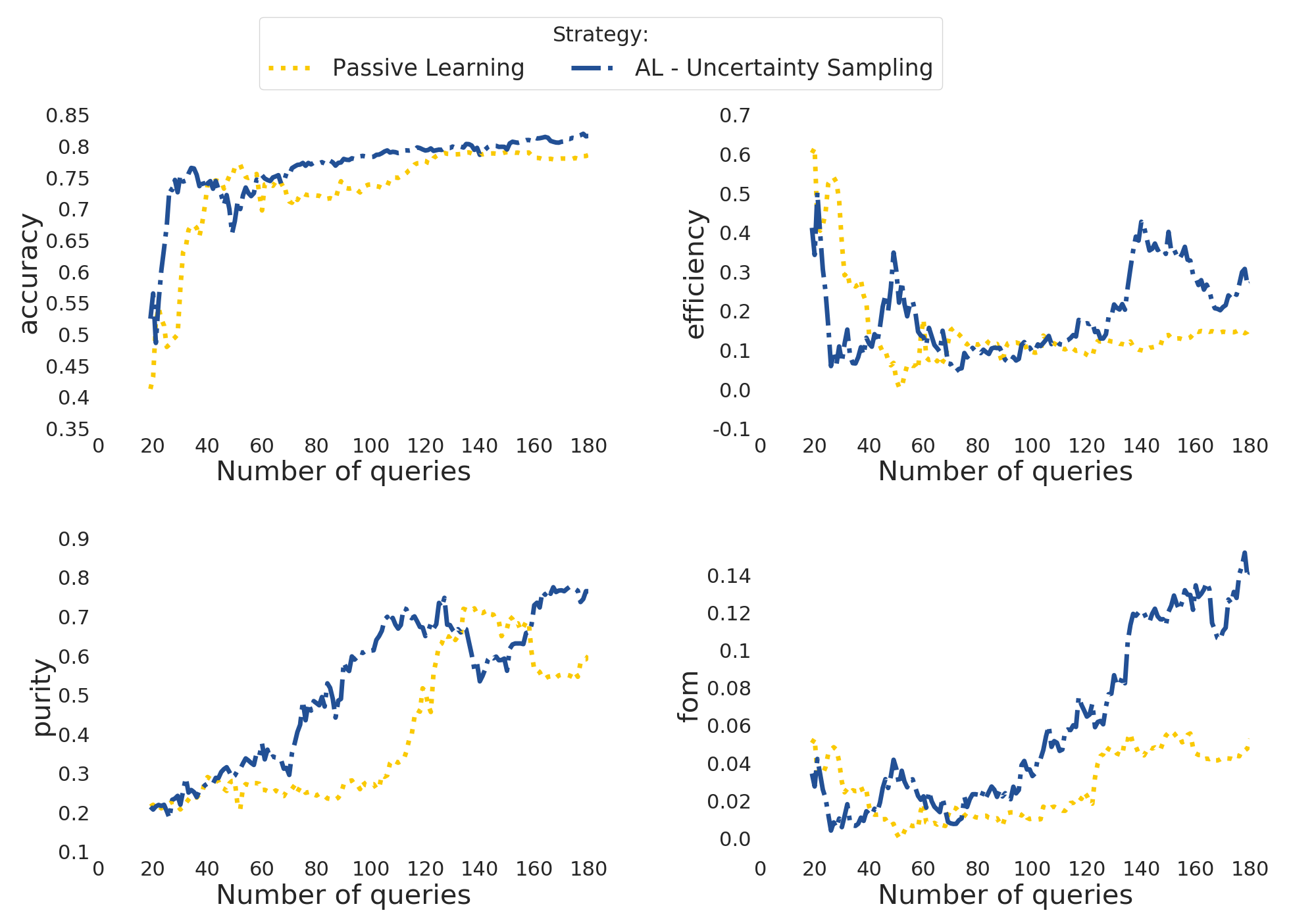
Once you ran one or more options, you can use the actsnclass.plot_results module, as described in the produce plots page. The result will be something like the plot below (accounting for variations due to initial training).

Warning

At this point there is no Canonical sample option implemented for the time domain module.