Feature Extraction
The first stage in consists in transforming the raw data into a uniform data matrix which will subsequently be given as input to the learning algorithm.
The current implementation of actsnclass text-like data from the SuperNova Photometric Classification Challenge
(SNPCC) which is described in Kessler et al., 2010.
Processing 1 Light curve
The raw data looks like this:
SURVEY: DES
SNID:   848233
IAUC:    UNKNOWN
PHOTOMETRY_VERSION: DES
SNTYPE:  22
FILTERS: griz
RA:      36.750000  deg
DECL:    -4.500000  deg
MAGTYPE: LOG10
MAGREF:  AB
FAKE:    2   (=> simulated LC with snlc_sim.exe)
MWEBV:   0.0283    MW E(B-V)
REDSHIFT_HELIO:   0.50369 +- 0.00500  (Helio, z_best)
REDSHIFT_FINAL:   0.50369 +- 0.00500  (CMB)
REDSHIFT_SPEC:    0.50369 +- 0.00500
REDSHIFT_STATUS: OK

HOST_GALAXY_GALID:   17173
HOST_GALAXY_PHOTO-Z:   0.4873  +- 0.0318


SIM_MODEL:  NONIA  10  (name index)
SIM_NON1a:      30   (non1a index)
SIM_COMMENT:  SN Type = II , MODEL = SDSS-017564
SIM_LIBID:  2
SIM_REDSHIFT:  0.5029
SIM_HOSTLIB_TRUEZ:  0.5000  (actual Z of hostlib)
SIM_HOSTLIB_GALID:  17173
SIM_DLMU:      42.276020  mag   [ -5*log10(10pc/dL) ]
SIM_RA:        36.750000 deg
SIM_DECL:      -4.500000 deg
SIM_MWEBV:   0.0256   (MilkyWay E(B-V))
SIM_PEAKMAG:   22.48  22.87  22.70  22.82  (griz obs)
SIM_EXPOSURE:     1.0    1.0    1.0    1.0  (griz obs)
SIM_PEAKMJD:   56251.609375  days
SIM_SALT2x0:   1.229e-17
SIM_MAGDIM:    0.000
SIM_SEARCHEFF_MASK:  3  (bits 1,2=> found by software,humans)
SIM_SEARCHEFF:  1.0000  (spectro-search efficiency (ignores pipelines))
SIM_TRESTMIN:   -38.24   days
SIM_TRESTMAX:    64.80   days
SIM_RISETIME_SHIFT:   0.0 days
SIM_FALLTIME_SHIFT:   0.0 days

SEARCH_PEAKMJD:   56250.734


# ============================================
# TERSE LIGHT CURVE OUTPUT:
#
NOBS: 108
NVAR: 9
VARLIST:  MJD  FLT FIELD   FLUXCAL   FLUXCALERR   SNR    MAG     MAGERR  SIM_MAG
OBS:  56194.145  g NULL   7.600e+00   4.680e+00   1.62   99.000    5.000   98.926
OBS:  56194.156  r NULL   3.875e+00   2.752e+00   1.41   99.000    5.000   98.953
OBS:  56194.172  i NULL   3.585e+00   4.628e+00   0.77   99.000    5.000   99.033
OBS:  56194.188  z NULL  -2.203e+00   4.463e+00  -0.49   99.000    5.000   98.983
OBS:  56207.188  g NULL  -7.008e+00   4.367e+00  -1.60   99.000    5.000   98.926
OBS:  56207.195  r NULL  -1.189e+00   3.459e+00  -0.34   99.000    5.000   98.953
OBS:  56207.203  i NULL   8.799e+00   6.249e+00   1.41   99.000    5.000   99.033
You can load this data using:
 1>>> from actsnclass.fit_lightcurves import LightCurve
 2
 3>>> path_to_lc = 'data/SIMGEN_PUBLIC_DES/DES_SN848233.DAT'
 4
 5>>> lc = LightCurve()                        # create light curve instance
 6>>> lc.load_snpcc_lc(path_to_lc)             # read data
 7>>> lc.photometry                            # check structure of photometry
 8          mjd band     flux  fluxerr   SNR
 9 0    56194.145    g   7.600    4.680   1.62
10 1    56194.156    r   3.875    2.752   1.41
11 ...        ...  ...      ...      ...   ...
12 106  56348.008    z  70.690    6.706  10.54
13 107  56348.996    g  26.000    5.581   4.66
14 [108 rows x 5 columns]
Once the data is loaded, you can fit each individual filter to the parametric function proposed by Bazin et al., 2009 in one specific filter.
1>>> rband_features = lc.fit_bazin('r')
2>>> print(rband_features)
3[159.25796385, -13.39398527,  55.16210333, 111.81204143, -20.13492354]
The designation for each parameter are stored in:
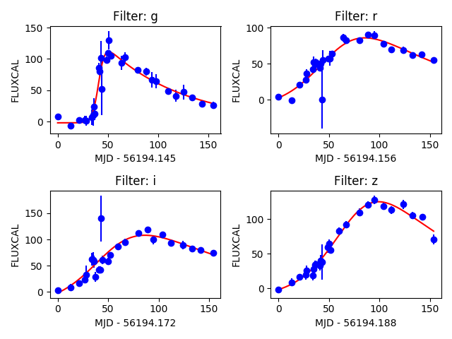
It is possible to perform the fit in all filters at once and visualize the result using:
1>>> lc.fit_bazin_all()                            # perform Bazin fit in all filters
2>>> lc.plot_bazin_fit(save=True, show=True,
3                      output_file='plots/SN' + str(lc.id) + '.png')   # save to file
Processing all light curves in the data set
There are 2 way to perform the Bazin fits for the entire SNPCC data set. Using a python interpreter,
1>>> from actsnclass import fit_snpcc_bazin
2
3>>> path_to_data_dir = 'data/SIMGEN_PUBLIC_DES/'            # raw data directory
4>>> output_file = 'results/Bazin.dat'                              # output file
5>>> fit_snpcc_bazin(path_to_data_dir=path_to_data_dir, features_file=output_file)
The above will produce a file called Bazin.dat in the results directory.
The same result can be achieved using the command line:
>> fit_dataset.py -dd <path_to_data_dir> -o <output_file>